Our previous research colloquia on COVID-19 consisted of 1) a preliminary sketch of a multi-scale thermodynamics paradigm (‘functional communication’) developed to analyze this phenomenon and 2) a graphical analysis of the economic attributes of the meso level of the crisis. Now, we combine these analyses in order to test the hypothesis about the success of economic shut-downs in stopping the spread of the virus by predicting the spread of the virus, based upon the functionality of the economy. Using a modified SEIR model of infections, we develop the transmission rates (betas) as functions of economic functionality via the proxy index of ‘relative job-loss,’ which was discussed at length in the previous colloquium. Through a basic graphical comparison of infection-rate and employment-rate we can see there is a definite dynamical relationship between them deserving a fuller functional explication.
Infection-Rate and Employment Comparison
Within the short-term, it is not possible to restructure employment in order to accommodate for the loss of proximate-communicative jobs, which must necessarily be halted in order to stop the spread of the infection. Economic-shutdown, as shown in the below figure (3) as total employment loss, was followed within a month with a decrease in the infection-rate. The positive effect of the economic shutdown was shown more clearly in NYC, where the infection-peak was much higher and the subsequent shutdown also more intensive, but nationally the job-loss was followed by a flattening of the infection-rate curve.
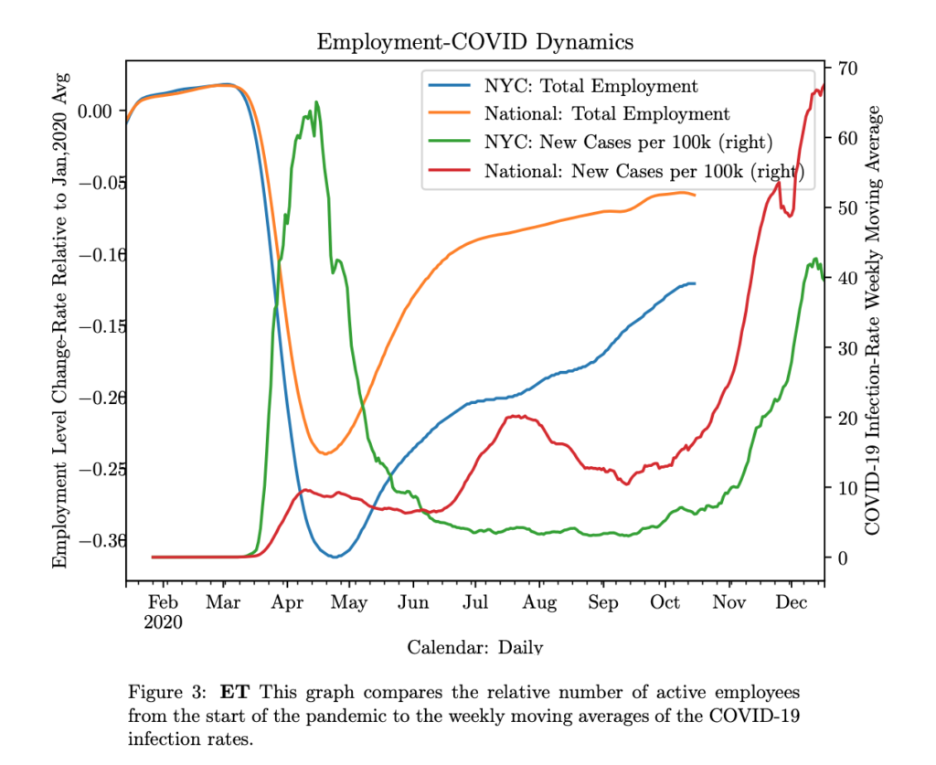
For both scales, NYC and nationally, a decrease in infection-rate was followed by a reopening of the economy after an apparent equilibrium was reached with 1/3 dysfunctionality (i.e. labor-side shut-down) in NYC and 1/4 dysfunctionality nationally. These may have been premature and the effects buffered by the fall moratorium on evictions.
Logistic Epidemic Model of COVID-19 Economic Dynamics
I follow a simplified and modified version of the SEIR model presented by Yang and Wang [2], using many of the parameter values discerned by them, but with the viral transmission rate functions based upon the continuous measurement of the economic shut-down, as given by employment-rate changes since January, 2020. In addition to the standard SEIR model, Yang and Wang’s model includes a novel environment variable of viral density to model the indirect pathway of the infection by surface contact and aerosol inhalation. Here I collapse the hospitalized subpopulation (H) into the infected subpopulation (I), which is thus any individual who has tested positive for coronavirus. The compartments in this model thus considered are Susceptible (S), Exposed (E), Infected (I), Recovered (R), and the Environment (V), thus forming a SEIRV model.
The Exposed population is an unmeasured quantity of those who have been exposed to the virus and are thus `infected’ but have not been tested, either because they are still in the incubation period ( days) or do not show any symptoms due to strong immune and respiratory systems. After this incubation period, a proportion of the exposed population (
 ) [4] develop symptoms and so get tested, while those of the post-incubation non-symptomatic population,
  , get tested at the same probability as the general population. Thus, given a testing rate of
  for the whole population, the post-incubation non-symptomatic get tested at a rate of
  . This is summarized as a post-incubation exposed testing rate of
  .
.
The Environment is included as a compartment since it holds viral density in the air as aerosol and in surfaces from those exposed or infected and can therefore transmit to the susceptible population via  .
.
System of Ordinary Differential Equations
![\[ 1. \frac{dS}{dt}=\Lambda + \mu S - \beta_E (t) SE - \beta_I (t) SI - \beta_V(t) SV \]](https://www.mathacademytutoring.com/wp-content/ql-cache/quicklatex.com-47c5a280c0a32b56829c92d680ac5dc3_l3.png "Rendered by QuickLaTeX.com")
![\[2. \frac{dE}{dt}=\beta_E (t) SE + \beta_I (t) SI + \beta_V(t) SV - (\alpha \chi (t)+\gamma_1 - \mu)E\]](https://www.mathacademytutoring.com/wp-content/ql-cache/quicklatex.com-781e0898e3902790b9348aa32c5316f7_l3.png "Rendered by QuickLaTeX.com")
![\[3. \frac{dI}{dt}=\alpha \chi (t)E - (\gamma_2 - \mu) I\]](https://www.mathacademytutoring.com/wp-content/ql-cache/quicklatex.com-418f78388a096ffa80ebdc8e9be0c237_l3.png "Rendered by QuickLaTeX.com")
![\[4. \frac{dR}{dt}=\gamma_1 E + \gamma_2I + \mu R\]](https://www.mathacademytutoring.com/wp-content/ql-cache/quicklatex.com-364e6335f9bbb3c71dbeb61cc655ef96_l3.png "Rendered by QuickLaTeX.com")
![\[5. \frac{dV}{dt}=\zeta_1 E + \zeta_2 I - \sigma V\]](https://www.mathacademytutoring.com/wp-content/ql-cache/quicklatex.com-e2ce43aba7faef51f6345298a3f1e33d_l3.png "Rendered by QuickLaTeX.com")
Parameter Estimation
In this model, the demographic parameters are the population flux rate ( ) and the natural birth-death rate
  . The birth rate (from 2017) for NYC is
  (per day) and the death rate for NYC is
  (per day) giving a natural birth-death rate of
  [5]. The population of NYC at the start of 2020 was
  . The population flux from NYC was negative this past year,
  (people per day) [6]. The 2020 birth-rate for the USA was
  and the death rate was
  [7], so
  , and the migration rate was
  . The population of the USA at the start of 2020 was
  .
.
The parameter estimations for the recovery rates and the environmental shedding/removal rates are from Yang, 2020. The recovery rate of exposed individuals is  per day, while of infected individuals is
  per day. The viral shedding rates (
 ) are the rates at which viral counts accumulate in the environment due to infected individuals. These are
  for exposed individuals and
  for infected individuals. The rate at which the virus is removed from the environment due to decay is
  .
.
The functions  are the direct human-to-human transmission rates between the exposed and susceptible individuals and between the infected and susceptible individuals, respectively, while represents the indirect environment-to-human transmission rate between the environment and susceptible individuals. For each transmission coefficient we separate them into their biological invariant coefficients measured from the ‘normal’ conditions of viral propagation,
  , although these may have possibly increased over time due to mutations, and their social dynamic components based upon the functional communicativity of the populations’ sociality given mostly by health policies and their compliance. Most likely,
  although the virus takes some time to replicate during the incubation period until the person is fully contagious. For the betas of the 3 transmission compartments, E, I, & V, we can formulate them functionally through the parallel expressions:
![\[\beta = \beta_0 f(t) g(t)\]](https://www.mathacademytutoring.com/wp-content/ql-cache/quicklatex.com-6e401a30c2014acc8a3f04361534e819_l3.png "Rendered by QuickLaTeX.com")
 is the macro functional-communicativity of the society and
  is the micro functional-communicativity of an average individual in the society, where both range between 0 for non-functional and 1 for normal (pre-pandemic), full, or natural functionality (i.e.
  ). can be functionalized via the economic subsystem by the relative job loss,
  , as
, as  and by the infection-rate,
  , in terms of fear-based compliance , as
  , where
  is a positive elasticity constant for the fear-sentiment sensitivity to compliance for the population. This set up is form-wise similar to Yang & Wang but differs in that is now a continuously-changing variable, rather than null, constant, or linear based upon the period policy, and is a function of the absolute infection-rate rather than relative to a period baseline.
In order to test the economic shut-down hypothesis, it remains thus to test how well it fits the data, which will be the subject of the next research colloquium.
References
- Data from Opportunity Insights’ Economic Tracker database available at \url{tracktherecovery.org}, using the two specific tables, “Employment Combined – National – Daily” and “Employment Combined – City – Daily” for Figure 1 and 2, where active employment numbers were collected from Paycheck, Intuit, Earnin, and Kronos.
- Chayu Yang and Jin Wang, “Modeling the Transmission of COVID-19 in the US – A Case Study.” Infectious Disease Modelling, Dec. 30 2020.
- Manotosh Mandal, et. al. “A model based study on the dynamics of COVID-19: Prediction and control.” Chaos, Solitons, and Fractals 136 (2020) 109889.
- Daniel P. Oran, Eric J. Topol. “Prevalence of Asymptomatic SAR-CoV-2 Infection.” A Narrative Review. Annals of Internal Medicine. 1 Sept. 2020. https://doi.org/10.7326/M20-3012.
- https://www1.nyc.gov/site/doh/data/data-sets/vital-statistics-data.page
- https://www.reuters.com/article/usa-economy-nyc-idUSKBN28P1Q8
- https://www.macrotrends.net/countries/USA/united-states/population