Limit of a Function: Introduction – Calculus

by ms-academy | Sep 12, 2021 | Math Learning

Table of Contents

In order to study a function and its behavior and properties, an important step is to find out the limits of the function on the ends of its domain of definition. In this article, we will introduce the idea of limits and the different cases that we can come across.

Introduction

We saw in a previous article, an introduction to functions and some of their properties, in this blog post we will learn about function’s limits, where we will try to the behavior of the function near infinity and near specific real values (i.e., the values for who the function isn’t defined), in other terms, we try to determine the function value when approaching the extremities of its domain of definition.

The idea of limits:

To better introduce the idea of limits, let’s take a look at some examples:

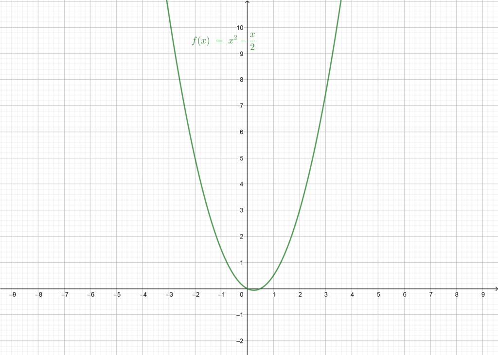
Example 1: Let’s the function $f$ be defined as follow:

$f(x)=x^{2}-\dfrac{x}{2}$

The domain of the function $f$ is $D_{f}=\mathbb{R}$ .

Let’s evaluate the function $f$ when the values of $x$ go bigger and bigger

$x$	1	5	10	$10^2$	$10^3$
$f(x)$	0.5	22.5	95	9950	999500

We notice that, as the value of $x$ increase, the value of the $f(x)$ increases as well, so we can predict that as the value of $x$ become bigger and bigger, the value of the function $f$ goes bigger and bigger too, meaning that as $x$ approaches infinity (infinitely big) the value of $f(x)$ approaches $+\infty$ as well. In this case, we can use the notation:

$\lim_{x\rightarrow+\infty}f(x)=+\infty$

And we read the limit of the function $f$ as $x$ approaches $+\infty$ , is $+\infty$ .

Here is the graph of the function $f$ for a better illustration:

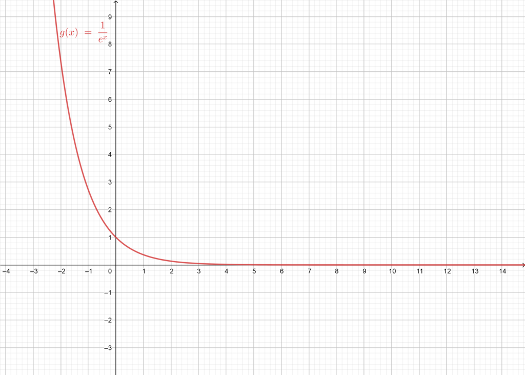
Example 2:

We have the function $g$ defined as:

$g(x)=\dfrac{1}{e^{x}}$

The domain of the function $g$ is: $D_{g}=\mathbb{R}$ .

Let’s evaluate the function $g$ as $x$ takes bigger and bigger values:

$x$	1	5	10	$10^2$	$10^3$
$g(x)$	0.36787944117	0.00673794699	0.00004539992	3.720076e-44	(To close to zero that the calculator shows exactly 0)

We can easily notice that as $x$ increases in value the value of $g(x)$ goes closer and closer to 0, so we can predict that as $x$ approaches infinity the value of the function $g$ approaches 0, and we note:

$\lim_{x\rightarrow+\infty}g(x)=0$

So, From the two previous examples, we conclude that a limit of a function can a real number or $\pm\infty$ .

Here is the graph representing the function $g$ , where we can see the graph approaching the X-axis $(y=0)$ as $x$ goes towards infinity.

Example 3:

Let’s consider the function $h$ defined as follow:

$h(x)=\dfrac{1}{x}$

We have the domain of the function $h$ is $D_{h}=\mathbb{R^{*}}=]-\infty;0[\cup]0;+\infty[$ .

We know that the function h isn’t defined for $x=0$ (because we can’t divide by 0), but let’s try and see the values of $h(x)$ as $x$ approaches 0 with both greater and less than 0, meaning we evaluate $h(x)$ when $x$ approaches 0 from the right side (i.e., $x>0$ ), and when $x$ approaches 0 from the left side (i.e., $x<0$ ).

Let’s start with evaluating $h(x)$ as $x$ gets closer and closer to zero with greater values:

$x$	1	0.5	0.1	0.01	0.001	0.0001	0.00001
$h(x)$	1	2	10	100	1000	10000	100000

We can clearly notice that as $x$ gets closer and closer to zero with greater values, the values of the function $h$ become bigger and bigger, we can predict then that it keeps increasing in value towards $+\infty$ , in other terms as $x$ approaches 0 with greater values, $h(x)$ tend to $+\infty$ , and we note:

$\lim_{x\rightarrow 0^{+}}h(x)=+\infty$

And we read: the limit of the function $h$ as $x$ approaches 0 with greater values (or as $x$ approaches 0 from the right side) is $+\infty$ .

Now let’s evaluate $h(x)$ as $x$ approaches 0 with values less than zero:

$x$	-1	-0.5	-0.1	-0.01	-0.001	-0.0001	-0.00001
$h(x)$	-1	-2	-10	-100	-1000	-10000	-100000

This time, notice that the value of the function $h$ gets smaller and smaller, as $x$ gets closer and closer to 0 with smaller values i.e., from the left side, so this way we can predict that $h(x)$ will keep decreasing towards $-\infty$ , meaning that as $x$ approaches 0 with smaller values, $h(x)$ tends to $-\infty$ , and we note:

$\lim_{x\rightarrow 0^{-}}h(x)=-\infty$

Here is the graph of the function $h$ , notice that the graph goes up to $+\infty$ if we get closer to 0 from the right side, and it goes down to $-\infty$ if we get closer to 0 from the left side.

Let’s summarize what we learned:

Finding the limit of a function is to determine its value tendency when $x$ approaches infinity or a real number (usually a value at the extreme of the function’s domain for which the function is not defined).

We evaluate limits for when $x$ approaches the ends on the domain of definition of a function, otherwise, if we want to evaluate the function for a value of $x$ inside the domain, we just calculate $f(x)$ , but for the values at the extremes of the domain, whether they are a real number or infinity, we cannot calculate them and that why we try to find the limits.

For example, we cannot just evaluate $f(\pm \infty)$ because infinity is not a number, infinity is an idea, a concept, so instead, we calculate the limit of the function $f$ when $x$ goes to infinity.

Same thing for a value of $x$ on the extreme of the domain and for which the function isn’t defined, for example, a function $f$ defined on a domain $D_{f}=]-\infty;x_{0}}[\cup ]x_{0};+\infty [$ , we know that $x_{0}$ doesn’t belong in the domain of $f$ so we cannot evaluate $f(x_{0})$ , instead, we calculate the limit of the function $f$ when $x$ approaches the value of $x_{0}$ . In this case, we have two limits to determine, one for when $x$ approaches $x_{0}$ with greater value (i.e., $x_{0}=x+\varepsilon$ where $\varepsilon$ is very small) or in other terms from the right side; and the second for when $x$ approaches $x_{0}$ with smaller values (i.e., $x_{0}=x-\varepsilon$ where $\varepsilon$ is very small) or in other terms from the left side.

Finite and infinite limit when approaching infinity:

Finite limit

Definition 1: Finite limit on $+\infty$ or $-\infty$ :

Suppose $f$ a function defined on the domain $D_{f}=[x_{0};+\infty[$ and $l$ a real number.

To say that the limit of $f$ on $+\infty$ is $l$ is to say that every open domain containing $l$ contains all the values of $f(x)$ for $x$ big enough. We write

$\lim_{x\rightarrow+\infty}f(x)=l$

And we read $f(x)$ tends to $l$ when $x$ tends to $+\infty$ .

Explanation:

To say that the limit of $f$ as $x$ tends to $+\infty$ is $l$ , means that $f(x)$ becomes very close to $l$ and therefore the value $f(x)$ lies in the interval $]l-\varepsilon;l+\varepsilon[$ , with $\varepsilon$ a small real number, or in other terms $\vert f(x)-l\vert<\varepsilon$ .

Remarque: we get a similar definition and result for $-\infty$ (i.e., for $f$ defined on $]-\infty;x_{0}]$ and $x$ tends to $-\infty$ ).

Examples:

$\lim_{x\rightarrow+\infty}\dfrac{1}{\sqrt{x}}=0 \;\;\;\;\; \lim_{x\rightarrow+\infty}\dfrac{1}{e^{x}}=0 \;\;\;\;\; \lim_{x\rightarrow+\infty}\left( \dfrac{1}{x}+3 \right)=3$

Infinite limit

Definition 1: Infinite limit on $+\infty$ or $-\infty$ :

Suppose $f$ a function defined on the domain $D_{f}=[x_{0};+\infty[$ and $l$ a real number.

To say that the limit of $f$ when $x$ tends to $+\infty$ is $+\infty$ , means that for a real number $A$ with $A\in \mathbb{R}$ , every interval $[A;+\infty[$ contains all the values of $f(x)$ for $x$ big enough. We write

$\lim_{x\rightarrow+\infty}f(x)=+\infty$

And we read $f(x)$ tends to $+\infty$ when $x$ tends to $+\infty$ .

Definition 2:

Suppose $f$ a function defined on the domain $D_{f}=[x_{0};+\infty[$ and $l$ a real number.

To say that the limit of $f$ when $x$ tends to $+\infty$ is $-\infty$ , means that for a real number $B$ with $B\in \mathbb{R}$ , every interval $]-\infty;B]$ contains all the values of $f(x)$ for $x$ big enough. We write

$\lim_{x\rightarrow+\infty}f(x)=-\infty$

And we read $f(x)$ tends to $-\infty$ when $x$ tends to $+\infty$ .

Remarque: we get two similar definitions and result for $-\infty$ (i.e., for $f$ defined on $]-\infty;x_{0}]$ and $x$ tends to $-\infty$ ).

Examples:

$\lim_{x\rightarrow+\infty}\sqrt{x}=+\infty \;\;\;\;\; \lim_{x\rightarrow+\infty}e^{x}=+\infty \;\;\;\;\; \lim_{x\rightarrow+\infty}x^{2}+3x-1=+\infty$

Finite and infinite limit when approaching a real value:

Finite limit when approaching a real value:

Definition:

Suppose $f$ a function defined on the domain $D_{f}=]-\infty;x_{0}[\cup]x_{0};+\infty[$ and $l$ a real number.

To say that the limit of $f$ when $x$ tends to $x_{0}$ is equal to $l$ , means that every open interval containing $l$ contains all the values of $f(x)$ for $x$ big enough. We write

$\lim_{x\rightarrow x_{0}}f(x)=l$

And we read: $f(x)$ tends to $l$ when $x$ tends to $x_{0}$ .

We distinguish two cases, the first is when $x$ tends to $x_{0}$ with greater values (or in other terms from the right side) and we note:

$\lim_{x\rightarrow x_{0}^{+}}f(x)=l$

And the second case, when $x$ tends to $x_{0}$ with smaller values (or in other terms from the left side) and we note:

$\lim_{x\rightarrow x_{0}^{-}}f(x)=l$

Let’s take a look at an example for better understanding:

We have the function $f$ defined on $\mathbb{R}^{*}=]-\infty;0[\cup]0;+\infty[$ as follow:

$f(x)=\dfrac{\sin(x)}{x}$

If we take a look at the graph of the function $f$ , we notice that as $x$ approaches 0 the value $f(x)$ approaches 1, and if we zoom the graph or if we use a table to calculate values as $x$ approaches 0 then we can see that we can get $f(x)$ as close to 1 as we want if we get $x$ close enough to 0. Therefore, we have:

$\lim_{x\rightarrow0}\dfrac{\sin(x)}{x}=1$

Infinite limit when approaching a real value:

Definition: Suppose $f$ a function defined on the domain $D_{f}=]-\infty;x_{0}[\cup]x_{0};+\infty[$ .

To say that the limit of $f$ when $x$ tends to $x_{0}$ is $+\infty$ , means that for a real number $A$ with $A\in \mathbb{R}$ , every interval $[A;+\infty[$ contains all the values of $f(x)$ for $x$ big enough. We write

$\lim_{x\rightarrow x_{0}}f(x)=+\infty$

And we read: $f(x)$ tends to $+\infty$ when $x$ tends to $x_{0}$ .

We distinguish two cases, the first is when $x$ tends to $x_{0}$ with greater values (or in other terms from the right side) and we note:

$\lim_{x\rightarrow x_{0}^{+}}f(x)=+\infty$

And the second case, when $x$ tends to $x_{0}$ with smaller values (or in other terms from the left side) and we note:

$\lim_{x\rightarrow x_{0}^{-}}f(x)=+\infty$

Here is an example for better understanding:

The function $g$ is defined on the interval $D_{g}=]-\infty;0[\cup]0;+\infty[$ as follow:

$g(x)=\dfrac{1}{x}$

If we take a look at the graph $(G_{g})$ we can clearly notice that as $x$ approaches 0 with greater value i.e., from the right side, the value of $f(x)$ tends to $+\infty$ , so we write:

$\lim_{x\rightarrow 0^{+}}\dfrac{1}{x}=+\infty$

Also, we can see that as $x$ approaches 0 with smaller values i.e., from the left side, the value of $g(x)$ tends to $-\infty$ , so we write:

$\lim_{x\rightarrow 0^{-}}\dfrac{1}{x}=-\infty$

Now why don’t you try it yourself, in the following graph of the function $g$ , you can slide the two points $x^{+}$ and $x^{-}$ on the X-axis, and approach 0 as close as you want while noticing the value of $y=f(x)$ goes to infinity with different signs
<span style="display: inline-block; width: 0px; overflow: hidden; line-height: 0;" data-mce-type="bookmark" class="mce_SELRES_start"></span>

Conclusion:

We learned in this article the idea of limits and how it helps us understand the behavior of a function near the edges of its domain of definition. this is just an introduction we still have much more to learn and

Surely you want more fun with limits, so check out this random rational functions generator, as its name suggests it randomly generate a rational function (a quotient of two polynomial functions) and draws its graph. Take a look and enjoy graphicly seeing the different limits of these functions on their domains. Have Fun!!!!!

You want to learn more fun subjects, check the post about Functions and some of their properties, or the one about How to solve polynomial equations of first, second, and third degrees!!!!!

And don’t forget to join us on our Facebook page for any new articles and a lot more!!!!!

← PREVIOUS NEXT →

Limit of a Function: Introduction – Calculus

Introduction

The idea of limits:

Finite and infinite limit when approaching infinity:

Finite limit

Infinite limit

Finite and infinite limit when approaching a real value:

Finite limit when approaching a real value:

Infinite limit when approaching a real value:

Conclusion:

Blog Main

Categories

Recent Posts

Archives

Archives

Categories

Meta