Probability theory – Conditional Probability

by ms-academy | Nov 1, 2021 | Math Learning

Table of Contents

Hello again!!! It is time to continue our journey in the field of probability theory; So, after introducing probability theory, the different types of probability and its axioms, and after presenting the basic terminology and how to evaluate the probability of an event in the simplest cases in the previous articles, in this one we will learn about conditional probability and the formula for evaluating the conditional events alongside some illustrating examples. So, without further ado let the fun begin!!!

Introduction

We learned previously that calculating the probability of an event is simple, knowing the sample space and the favorable outcomes. It is straightforward, all it takes dividing the number of favorable outcomes by the total number of outcomes. But what if the event we are evaluating its probability is related to another event, or what if we receive new information from the previous trials, does this information change or affect the probability of the event we are investigating?! Does all information affect the probability of the event we are currently investigating?! And how to evaluate an event if it is dependent on another one?! We will answer all these questions and more in this article.

First, we will take a look at the different types of events and the various possible types of relations between two events, after that we will proceed to introducing the concept of conditional probability and its meaning, we will introduce the formula of conditional probability alongside an explanation to make it trivial and easy to grasp and of course, we will take a look at some illustrating examples to strengthen and test our understanding of the conditional probability, afterword we will present the main properties of conditional probability, also we will introduce the Bayes’ theorem, and finally we will learn about the usage and applications of conditional probability in the different sciences and fields.

Types of events

Sure and impossible events:

We call a “sure event” every event that its probability is equal to 1, meaning, and as the name suggests, that we are sure of the occurrence of this event. On the other hand, we call an “impossible event” every event that its probability is equal to 0, in other terms, and as the name suggests as well, we are certain that the event will not occur.

An example of a sure event is the event that the sum of rolling of two dice is less or equal to 12.

An example of an impossible event is the event of getting a number greater than 6 on a roll of a die.

Simple events:

We call a “simple event” all event that is a one and only one element of the elements of the sample space.

For example, the event of getting the number 5 from a roll of a fair die is a simple event since 5 is one element of the sample space $S=\lbrace 1,2,3,4,5,6\rbrace$ , but if we take the event $E$ of getting a prime number as a result of a roll of a die, this event is not a simple event since the event E is composed of multiple elements of the sample space $S$ , so if we write the event E as a set we get: $E=\lbrace 2,3,5\rbrace$ meaning that it has three elements of the sample space and not just one.

Compound events:

This is the opposite case of the simple space, we call a “compound event” every event that has more than one element of the sample space, in other terms a compound event is an event that contains multiple outcomes of the possible outcomes of the sample space.

For example, the event of getting an odd number after the rolling of two fair dice is a compound event since it contains six elements of the sample space, so if write the sample space we get $S=\lbrace 2,3,4,5,6,7,8,9,10,11,12\rbrace$ and we have the set of the event $E$ can be written as $E=\lbrace 3,5,7,9,11\rbrace$ , we can clearly see that the event $E$ is a compound one.

But, if we take the event of getting a “Tail” after a fair coin toss, this event is not a compound one since it has only one element of the sample space $S=\lbrace \text{Head},\text{Tail} \rbrace$ (and therefore it is a simple event).

Independent events:

We describe events as “independent” in the case where the happening of any event doesn’t affect the chances of occurrence of any other event, and we call them “independent events”. In other terms, for two events to be called independent one must have no influence on the chances of occurrence of the other.

For example, if we take the case of rolling a fair die, we know that every roll is completely unaffected by the result of the previous roll, so the chances of occurrence of the number 2 for instance, is the same no matter the number we got from the last roll.

Another example is the toss of a fair coin, it is clear that every toss is completely separate from the next one, and we know that every toss is not affected whatsoever by the result of the previous toss, so if we take for instance the chances of getting “Tail” after getting fifty-three times in a row the result “Head”, the chances are still the same, and we still have $P(\text{``Tail''}) = P(\text{``Head''}) = 50\%$ .

Another one is getting a free lunch at your favorite restaurant and the weather becoming rainy; winning the lottery and the occurrence of a solar eclipse that day; or raining and running out of milk.

Dependent events:

We describe events as “dependent” in the case where the probability of occurrence of any event is affected by the happening of another event and we call them “dependent events”. In other terms, for two events to be called dependent one must have an influence on the chances of occurrence of the other.

So, one good example of dependent events is the following: if we consider having an urn containing 4 white balls, three blue ones, and 7 purple ones, if we take out a ball without looking and without returning it back to the urn, and we consider and we consider the event A of taking out a purple ball, well, at the first take out we have the probability of this event as usual which is the number of favorable outcomes divides by the total number of the possible outcomes, so we get:

$P(A)=\dfrac{7}{14}=50\%$

But if we consider a second take out, knowing that we took a purple ball in the first time, the probability is affected, it is no more $50\%$ because when we took out one ball, we didn’t put it back in the urn and therefore we have now 6 purple instead of 7 and we have a total of 13 balls instead of 14.

Another example of two independent events is the following: suppose we have a giveaway and we have 100 participants, the giveaway has to parts: at the beginning, 50 people will be chosen randomly to win a headphone for each, and after that 3 lucky people from the winners of the headphones will win an iPhone 13 Pro. Well, notice that the event of winning an iPhone 13 pro is dependent on the event of winning the headphones since in order to be considered for the iPhone giveaway you need to be already a winner of the headphone. In other terms, the chance of winning an iPhone 13 pro is affected by the chance of winning a headphone.

Mutually exclusive events:

We describe two events as “mutually exclusive”, if the occurrence of one event implies the non-occurrence of the other one, meaning that if one event happens, we know for sure that the other one didn’t, and vise-versa. In other terms, the occurrence of one event excludes the occurrence of the other and hence they are called “mutually exclusive events”.

For example, if we have the experiment of rolling of a fair die and if we consider the two events $E_{1}$ and $E_{2}$ as follow:

$E_{1}$ : the event of getting an odd number.

$E_{2}$ : the event of getting an even number.

Also, we write sample space and the two events $E_{1}$ and $E_{2}$ in the form of sets, we have:

$S=\lbrace 1,2,3,4,5,6\rbrace$ , $E_{1}=\lbrace 1,3,5\rbrace$ and $E_{2}=\lbrace 2,4,6\rbrace$ .

Then we know that the two events $E_{1}$ and $E_{2}$ are mutually exclusive since that we can’t have a number as a result of a roll of a die that is at the same time odd and even. And also, we know that the two events are mutually exclusive by looking at the elements of each event and noticing that there is no common element and thus they can’t occur at the same time (The intersection of $E_{1}$ and $E_{2}$ is the empty set).

Another example is the toss of a coin, we have one of two events: “Head” or “Tail” and the occurrence of one of them implies the non-occurrence of the other since we can’t have the two results together.

Some other examples are: winning and losing the lottery, driving forward and backward, …etc.

Complementary events:

Suppose we have a sample space $S$ and an event $E_{1}$ , we call the “complementary event” of $E_{1}$ , the event $E_{2}$ that contains all the elements of the sample space other than the ones contained in $E_{1}$ . In other terms, the complementary event of $E_{1}$ is the set of the remaining elements of S if we remove the ones that are in $E_{1}$ .

We can write $E_{2}=S-E_{1}$ .

Notice that the two events $E_{1}$ and $E_{2}$ are mutually exclusive.

For example, if we consider the event $E_{1}$ of having a number less or equal than 4 as a result of a rolling of a fair die. We have the sample space $S$ : $S=\lbrace 1,2,3,4,5,6\rbrace$ , and we have the event E1 can be written as $E_{1}=\lbrace 1,2,3,4\rbrace$ , thus we have the complementary event of $E_{1}$ as follow:

$E_{2}=S-E_{1}$ ; $E_{2}=\lbrace 5,6\rbrace$ .

Another example is having the experiment of rolling a fair die and considering the event of getting an even number, we know that the elements that are in the sample space and not even can’t be anything other than odd numbers, and therefore the complementary event of getting an even number as a result of the roll is the event of getting an odd number.

After taking a look at the different types of events let us now learn what is conditional probability.

Conditional probability

Conditional probability is defined as the probability of occurrence of an event knowing that another event has already happened, different from performing the experiment for the first time, in the case of conditional probability we have additional information that is related and can affect the evaluation of the chances of an event occurring. Knowing this new information gives us a new insight and pushes us to calculate the probability in question while taking the new information into consideration. Bear in mind that conditional probability doesn’t imply that there is always a causal relation in the midst of the two events, there are several cases depending on the types of events and the relation between them. Conditional probability opens the question: as we get new and additional information does this allow gives us the possibility and the potential of reevaluating the probabilities we actually have and get a better estimation of the chances of occurrence of the coming events?!

Thus, the goal of conditional probability is finding the probability of an event given that or knowing that another event has occurred.

If we have two events $A$ and $B$ the probability of occurrence of $A$ , provided the information that $B$ has already happened is noted by the notation: $P(A\vert B)$ and we read: the probability of the event $A$ given the event $B$ .

Let’s take a quick example: If we have an urn containing four balls: white, blue, orange, and purple, in this experiment we draw without returning the drawn ball.

And we want to evaluate the probability of drawing the orange ball after already drawing the purple one.

First, we note the following events:

$A$ : The event of taking out the purple ball.

$B$ : The event of taking out the orange ball.

Now, and assuming that the balls have the same chance of getting taken out, we have that the probability of drawing the purple ball is $P(A)=25\%$ .

But assuming that the event of picking the purple ball occurs, now we have three remaining balls which imply a change of the probability of picking one of them it is no more $25\%$ , instead it is now $\dfra{1}{3}\simeq 33.33\%$ .

So the probability of drawing the orange ball after already drawing the purple one is $25\%\times 33.33\%\simeq 8.33\%$ .

For more understanding let’s take a look at this example: Suppose that a fair die has been rolled and we want to evaluate the probability of getting a 2. Typically and since the die is fair the probability is $P(\lbrace 2\rbrace)=\dfrac{1}{6}$ . But if we are given the information that the resulting number from the roll is an even number! Now we do not still consider the sample space as if it still has all six possible outcomes, but instead, we now have only three possibilities which are 2,4, and 6, and thus the probability becomes equal to $\dfra{1}{3}$ instead of $\dfrac{1}{6}$ .

Now suppose we got different information, we got informed that the resulting number of the roll is an odd number! In this case, we know that the chances of getting a 2 are impossible meaning $P(\lbrace 2\rbrace)=0$ .

This demonstrates how the new information can influence the probability and help to get a better and more accurate estimation of the occurrence of the event in question.

The formula of conditional probability

The conditional probability has a formula that helps us to evaluate the wanted probability easily, let’s take a look at it:

Suppose that we have two events $A$ and $B$ , the conditional probability $P(A\vert B)$ is given as follow:

$P(A\vert B)=\dfrac{P(A\cap B)}{P(B)}$

Where:

$P(A\vert B)$ : the probability of the event $A$ given the event $B$ .

$P(A\cap B)$ : the probability of the intersection of $A$ and $B$ .

$P(B)$ : the probability of $B$ .

The formula of the conditional probability is derived from the multiplication rule (also called chain rule), which, if we are using a tree diagram, means that in order to evaluate the probability of an event at any point of the tree diagram by multiplying the probabilities of the branches leading to that point. This also shows how useful and important the tree diagram is for conditional probability problems and for the probability theory in general. The multiplication rule is given by the following formula:

$P(A \cap B) = P(A) P(B\vert A)$

And therefore, by dividing the formula by $P(A)$ we derive the formula for the conditional probability $P(B\vert A)$ .

Here is a tree diagram illustrating the multiplication rule:

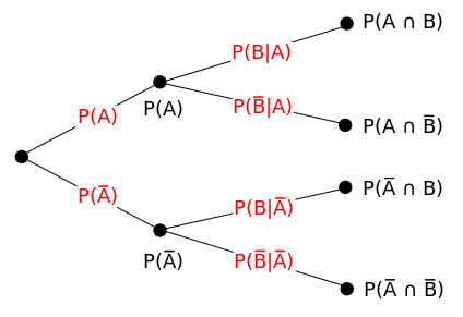
So, an easy visual way to calculate conditional probability is by using the tree diagrams.

Conditional probability for independent events:

From the definition we saw of independent events, we know that one event doesn’t have any effect on the probability of occurrence of the other, and therefore the conditional probability of the events A and B and knowing that the two events are independent is given as follow:

$P(A\vert B)=P(A),$

$P(B\vert A)=P(B).$

Conditional probability for mutually exclusive events:

As we learned earlier, mutually exclusive events can’t happen at the same time, and that the occurrence of one implies the non-occurrence of the other, and thus we have the conditional probability of two mutually exclusive events $A$ and $B$ is given as follow:

$P(A\vert B)=0,$

$P(B\vert A)=0.$

Law of total probability:

By using the multiplication rule we can evaluate the probability of various cases, and thus by using the multiplication rule we can derive what is called the Law of total probability.

Let’s suppose that we have a sample space $S$ and that it is divided into three disjoint events noted $X$ , $Y$ , and $Z$ ; therefore we have the following result for any given event $A$ :

$P(A)=P(A \cap X) +P(A \cap Y) +P(A \cap Z)$

And by replacing the terms on the right using the multiplication rule we get the expression for the law of total probability:

$P(A)= P(A\vert X) P(X) +P(A\vert Y) P(Y) +P(A\vert Z) P(Z).$

Properties of the conditional probability:

Here are a few properties of conditional probabilities:

Suppose we have three events $A$ , $B$ and $C$ , and we have $P(C)>0$ , we have the following properties:

$P(A^{c}\vert C)=1−P(A\vert C)$
$P(\emptyset \vert C)=0$
$P(A\vert C)\leq 1$
$P(A−B\vert C)=P(A\vert C)−P(A\cap B\vert C)$
$P(A\cup B\vert C)=P(A\vert C)+P(B\vert C)−P(A\cap B\vert C)$
if $A\subset B$ then $P(A\vert C)\leq P(B\vert C)$

Bayes’ theorem

The British mathematician Thomas Bayes from the 18^th century developed a mathematical formula that helps us to determine the conditional probability (also known as Bayes’ law or Bayes’ rule), this formula is given as follow:

Suppose we have two events $A$ and $B$ , and $P(B)>0$ , then:

$P(A\vert B)= \dfrac{P(A\vert B)P(B)}{P(A)}.$

This theorem is fundamental, important, and of great use in order to estimate the probability of an event based on new knowledge and information that may have a relation with the event in question. This helps us update the probabilities and estimations and get more accurate and updated predictions and revise the present ones knowing the new information.

Application of conditional probability

Conditional probability is one of the most important and fundamental concepts of the probability theory, and in many other fields and sciences since it deals with the idea of the existence of a relationship between the events that may cause a change or make a difference in the estimation of the probability of the events in question, and this idea of the existence of a relation between things is what is most common in sciences and in the real-life in general. Also, the Bayes’ theorem is widely used in various fields like statistics and finance, banking, sports, health care, and genetics to name just a few. And with the growing businesses dealing with huge data and information the importance of probability theory and its various branches is more and more clear and apparent.

Conclusion

Well, here we come to the end of this article, and after taking this fun journey with conditional probability and the different properties, and learning about the importance and usage of conditional probability in real life, it is safe to say that we are extremely excited to learn more about probability theory and wander through the world of probabilities!!! Don’t worry at all, more fun articles are coming soon!!!

In the meantime, you can take a look at some articles about limits and infinity like Limit of a function: Introduction, Limits of a function: Operations and Properties, Limits of a function: Indeterminate Forms, or the ones about Infinity: Facts, mysteries, paradoxes, and beyond or check the ones about Probability: Introduction to Probability Theory, or Probability: Terminology and Evaluating Probabilities !!!!!

There are also some articles about Set Theory like Set Theory: Introduction, or Set theory: Venn diagrams and Cardinality!!!!!

Also, if you want to learn more fun subjects, check the post about Functions and some of their properties, or the one about How to solve polynomial equations of first, second, and third degrees!!!!!

And don’t forget to join us on our Facebook page for any new articles and a lot more!!!!!

← PREVIOUS NEXT →