Continuity – Calculus

by ms-academy | Nov 8, 2021 | Math Learning

Table of Contents

Welcome again to another article!!! This time with a new article in Calculus, and the topic of our journey this time is Continuity; so, after introducing the concept of limits of a function, their properties, and the different operations on limits alongside presenting the indeterminate forms that we may encounter when evaluating limits and how to deal with them and work around them in order to determine the limit in question. We even learned about the interesting and strange Fun Facts – Infinity Facts, mysteries, paradoxes, and beyond in an entertaining blog post full of information, so make sure to check the previous article and to not miss any. Today we are taking a look at a new topic closely related to limits which is Continuity, in this article we will learn about the definition of continuity, how to determine if a function is continuous or not, and many more other things with some illustrating examples to grasp the content easily, now that we are eager to learn about continuity and with no further ado let the fun begin!!!

Introduction

In the previous article, we learned about how to study a function, and their domains of definition and codomains, a since we know that the domain of definition of a function is the set of possible values for which the function has an image or in other terms, but this may push ask some questions: does the graph of every function is formed of a single part or a single curved line?! Also, what about composite functions?!! How would their graphs look like, and does it always come in a signal part?!! Well, these questions and more will be answered by the end of this article.

At first, we will learn about the idea of continuity with some simple and easy definitions in addition to some rigorous mathematical definitions of the continuity of a function on a domain or at a single point of its domain, after that, we will learn about the three conditions necessary to verify the continuity of a function at a point and the various properties of continuity. Next, we will proceed to learn about the discontinuity of a function alongside the different types of discontinuity, afterword we will introduce the theorem of intermediate values all this alongside taking a look at some illustrating examples in order to have a better understanding of the subject.

Continuity of a function

Well, one of the simplest ways to define a continuous function is that a continuous function is any function that has the characteristic that its graph can be drawn with a pen without needing to lift the pencil from the page, so for a function to be continuous on a domain or an interval the graph must be one single curved line and having one part not multiple on this interval i.e. there are no holes, breaks or gaps, of course, this definition isn’t a formal mathematical one but is used to simply explain the concept in an easy way.

Continuity of a function at a point

For more formal, accurate, and a well mathematically put definition, we define the continuity of a function at a point as follow:

Definition 1:

Let $f$ be a function, let $D_{f}$ be its domain of definition, and let $a$ be a real number non isolated of $D_{f}$ ;

To say that the function $f$ continuous at the point $a$ , means that the limits of the function $f$ at the point $a$ is $f(a)$ .

Meaning:

$(f \text{ continuous at }a)\Leftrightarrow\lim_{x\to a}f(x)=f(a)$

For better understanding let’s take a look at some examples:

Example 1:

We have the function $f$ defined on the interval $[-2;2]$ as follow:

$f(x)=\begin{cases} -x, \;\;\; & x\in[-2;0]\\ \; x^{2}, \;\;\; & x\in[0;2] \end{cases}$

If we represent the function graphicly we get the following graph:

Notice the graph can be drawn without lifting the pen from the paper.

Therefore we can conclude that the function $f$ although being a composite function is continuous.

Let’s take a look at another example.

Example 2:

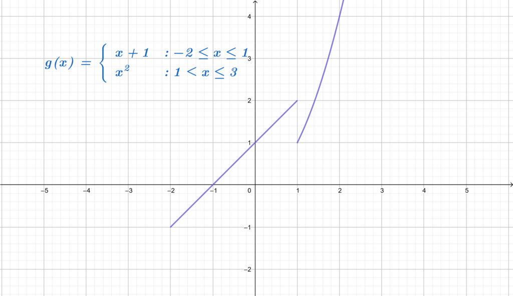
Let the function $g$ be defined as follow on the domain $[-2;3]$

$g(x)=\begin{cases} x+1, \;\;\; & x\in[-2;1]\\ x^{2}, \;\;\; & x\in]1;3] \end{cases}$

Here is the graph:

If we take a look at the graph of the function $g$ we clearly notice that the graph can’t be drawn without lifting the pen of the paper.

Also, if from the first and second examples we can deduce that composite functions can be continuous on their domain of definition.

In addition, we notice that in order for a function to be continuous at a point, this point must be contained in the domain of the definition of the function. Meaning that in order to use the definition above we assume the existence of $f(a)$ and $\displaystyle\lim_{x\to a}f(x)$ .

This last point leads us to another definition of the continuity of a function at a point, which is the following:

Definition 2: Continuity at a point:

$\lim_{x\to a}f(x)=f(a)\Leftrightarrow\lim_{x\to a^{-}}f(x)=f(a) \text{ and } \lim_{x\to a^{+}}f(x)=f(a)$

This means that in order for a function to be continuous at a point, the limits of $f$ when $x$ tends to a from both sides positive and negative side must be equal to $f(a)$ .

The tree conditions of continuity at a point:

From the previous examples, we can deduce the three conditions necessary in order for a function to be continuous, here they are:

Definition 2:

Suppose we have a function $f$ , we say that $f$ is continuous on a point $a$ , if and only if these conditions are verified:

$F(a)$ exists;
$\displaystyle\lim_{x\to a}f(x)$ exists;
$\displaystyle\lim_{x\to a}f(x)=f(a)$ .

Continuity of a function on an interval:

So, now that we defined what is continuity of a function at a given point of its domain of definition, we can now generalize the concept to define the notion of continuity of a function on an interval as follow:

We say that the function $f$ is continuous on an interval $I$ if and only if $f$ is continuous on every point of the interval $I$ .

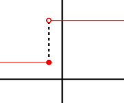
Continuity from the left:

We describe a function $f(x)$ as continuous from the left at the point $c$ if and only if:

$f(c)$ exists;
$\displaystyle\lim_{x\to c^{-}}f(x)$ exists;
$\displaystyle\lim_{x\to c^{-}}f(x)=f(c)$ .

A graph of a left-continuous function

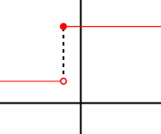
Continuity from the right:

We describe a function $f(x)$ as continuous from the right at the point $c$ if and only if:

$f(c)$ exists;
$\displaystyle\lim_{x\to c^{+}}f(x)$ exists;
$\displaystyle\lim_{x\to c^{+}}f(x)=f(c)$ .

A graph of a right-continuous function

Using this idea of continuity from the left and the right we can provide a definition for continuity on an interval.

Definition:

We say that a function $f(x)$ is continuous on a closed interval $[a,b]$ , if and only if, these condition are verified:

$f(x)$ is continuous on $[a,b]$ ;
$f(x)$ is continuous from the right at the point $a$ ;
And $f(x)$ is continuous from the left at point $b$ .

Let’s take a look at an example:

Let’s determine if the function $f(x)$ is continuous on the interval $[-4;4]$ , with $f$ defined as:

$f(x)=\sqrt{x^2-16}$

First we verify that $f$ is continuous on $I=[-4;4]$ :

We have $\displaystyle\forall c \in [-4;4] \lim_{x\to c}f(x)= \lim_{x\to c}\sqrt{x^2-16}=\sqrt{\lim_{x\to c}x^2-16}=\sqrt{c^2-16}=f(c)$

Therefor $f$ is continuous on $[-4;4]$ .

Second, we verify that $f$ is continuous from the right at the point $c=-4$ :

We have $\displaystyle\lim_{x\to -4^{+}}f(x)= \lim_{x\to -4^{+}}\sqrt{x^2-16}=\sqrt{\lim_{x\to -4^{+}}x^2-16}=0=f(-4)$

Therefor $f$ is continuous from the right at the point $c=-4$ .

Third, we verify that $f$ is continuous from the left at the point $c=4$ :

We have $\displaystyle\lim_{x\to 4^{-}}f(x)= \lim_{x\to 4^{-}}\sqrt{x^2-16}=\sqrt{\lim_{x\to 4^{-}}x^2-16}=0=f(4)$

Therefor $f$ is continuous from the left at the point $c=4$ .

So, the function $f$ is continuous on the closed interval $I=[-4;4]$

Some properties of continuity

It is important and necessary to know the main properties of continuity because knowing them will make deducing the continuity of some complicated function easier and faster than trying without the use of these properties, here they are:

Here are some of the main properties of the continuity of functions:

The addition: The addition of two functions $f$ and $g$ that are continuous on the interval $I$ (i.e. $f(x)+g(x)$ ) is a continuous function on $I$ .
The subtraction: the subtraction of two functions $f$ and $g$ that are continuous on the interval $I$ (i.e. $f(x)-g(x)$ ) is a continuous function on $I$ .
The scalar product: the product of a real number $k$ by a function $f$ that are continuous on the interval $I$ (i.e $k.f(x)$ ) is a continuous function on $I$ .
The product: the product of two functions $f$ and $g$ that are continuous on an interval $I$ (i.e. $f(x)\times g(x)$ ) is a continuous function on $I$ .
The division: we state two main cases:
the division of two functions $f$ and $g$ that are continuous on an interval $I$ (i.e. $\dfrac{f(x)}{g(x)}$ ) and with $g(x)$ different than 0 on $I$ , is a continuous function.
The division of two $f$ and $g$ that are continuous on an interval $I$ and with $g(c) = 0$ for $c\in I$ , is a discontinuous function.
Composite function: the composition of two functions $f$ and $g$ that are continuous on an interval $I$ is a continuous function.
The power: the power of a continuous function $f$ to $n$ where $n$ is appositive integer (i.e. $\left[f(x) \right]^{n}$ ) is a continuous function.
The root: the nth root of a continuous function $f$ where $n$ is a positive integer, is a continuous function.

These properties are easy to prove, so let’s take a look at a few proofs:

Let’s suppose that $f$ and $g$ are two continuous functions at a point $c$ .

We have $\displaystyle\lim_{x\to c}f(x)=f(c)$ (since $f$ is continuous at $c$ ),

And we have $\displaystyle\lim_{x\to c}g(x)=g(c)$ (since $g$ is continuous at $c$ ),

And we know that:

$\displaystyle\lim_{x\to c}[f(x).g(x)]= \lim_{x\to c}f(x). \lim_{x\to c}g(x)= f(c).g(c)$

Therefore, the product function is continuous

The same thing if we take the the summation or the subtraction of the functions:

$\displaystyle\lim_{x\to c}[f(x)+g(x)]= \lim_{x\to c}f(x)+ \lim_{x\to c}g(x)= f(c)+g(c)$

$\displaystyle\lim_{x\to c}[f(x)-g(x)]= \lim_{x\to c}f(x)- \lim_{x\to c}g(x)= f(c)-g(c)$

Example 1:

Let’s try to find out if the function $H$ is continuous:

$H(x)=\dfrac{x^2-9}{x^2-1}$

We have that the function $H$ is the division of two functions $f_{1}=x^2-9$ and $f_{2}=x^2-1$

Since these two functions are polynomials then we know that they are continuous on their domain of definition which is $\mathbb{R}$ for both of them.

Now, all we need is to know if the denominator can have a null value;

$F_{2}=x^2-1=0$ $x_{1}=1 \text{ or } x{2}=-1$

We have the denominator can be null for two values, therefore the function $H$ is discontinuous (discontinuous on the points 1 and -1).

Example 2:

These functions are continuous:

$f(x)= cos(x)+x$ ; $g(x)= \dfrac{x^2+1}{\cos x}$ ; $h(x)=\sin\left(\dfrac{1}{x}\right)$ .

Continuity of some known continuous functions:

Theorem:

Every Polynomial, Rational, Root, Exponential, Logarithmic, trigonometric, and inverse trigonometric function is a continuous function on its domain.

Discontinuity of a function

A discontinuous function is a function that isn’t continuous.

In simple and easy put words we say that a function is discontinuous if the graph of the function can’t be drawn without lifting the pen, meaning that the graph has at least two separated parts.

A more rigorous definition is that a discontinuous function at a point $c$ is a function that the limit from the left at the point $c$ is different from the limit of that function to the right at the point $c$ .

Meaning:

$\displaystyle \lim_{x\to c^{+}}f(x) diff \lim_{x\to c^{-}}f(x)$

Also, if a function isn’t defined at a point $c$ then it is discontinuous on every interval that contains the point $c$ .

Similarly to what we saw as conditions for a function to be continuous we can define conditions that are sufficient for a function to be discontinuous:

If $f(x)$ doesn’t exist at a point $c$ ;
If $\displaystyle\lim_{x\to c}f(x)$ doesn’t exist meaning: $\lim_{x\to c}f(x)\pm\infty$ ;
If $\displaystyle\lim_{x\to c^{+}}f(x)$ , $\displaystyle\lim_{x\to c^{-}}f(x)$ , and $f(c)$ are different.

Examples of discontinuous functions:

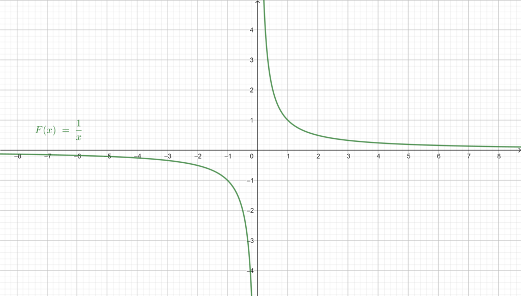
Example 1:

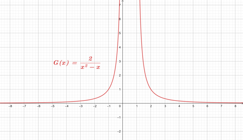
A known function that is discontinuous is the inverse function $\dfrac{1}{x}$

By looking at the graph, we can clearly notice that it is composed of two separated (i.e. disconnected) parts meaning it can’t be drawn without lifting the pen.

The point for which the function is discontinuous is 0, and we have the domain of the inverse function is $D=]-\infty;0[\cup]0;+\infty[$ .

Example 2:

Let’s have a look at the graph of the function $G$ :

$G(x)=\dfrac{2}{x^{2}-x}$

We have the domain of $G$ is $D=]-\infty;0[\cup]0;1[\cup]1;+\infty[$

Notice that the graph has three separated parts, similarly to the domain of definition that is composed of the union of three intervals.

Types of discontinuity:

we can distinguish three types of discontinuity based on the form of the discontinuous graph in question.

Jump discontinuity:

We say that a discontinuous graph has a jump discontinuity if the graph is detached at a point $c$ and the limits of the function to the right and to the left of $c$ are not the same i.e.:

$\displaystyle\lim_{x\to c^{+}}f(x) \diff \lim_{x\to c^{-}}f(x)$ and therefore $f(c)$ doesn’t exist.

Then $c$ is described as a jump discontinuity (or step discontinuity, or a discontinuity of the first kind).

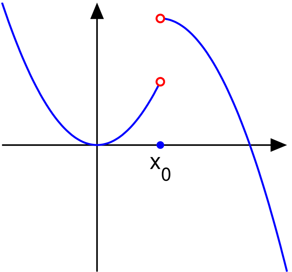
Here is an example of a graph of a function that has a jump discontinuity:

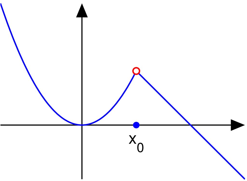
Removable discontinuity:

We say that a discontinuous graph has a removable discontinuity at a point $c$ if the limits from both sides left and right at the exists and if they are equal i.e. $\displaystyle\lim_{x\to c^{+}}f(x) =\lim_{x\to c^{-}}f(x)$ but they are different than $f(x)$ . in this case, the graph would look like a continuous graph except for a point detached point. Here is an example of a graph having a removable discontinuity:

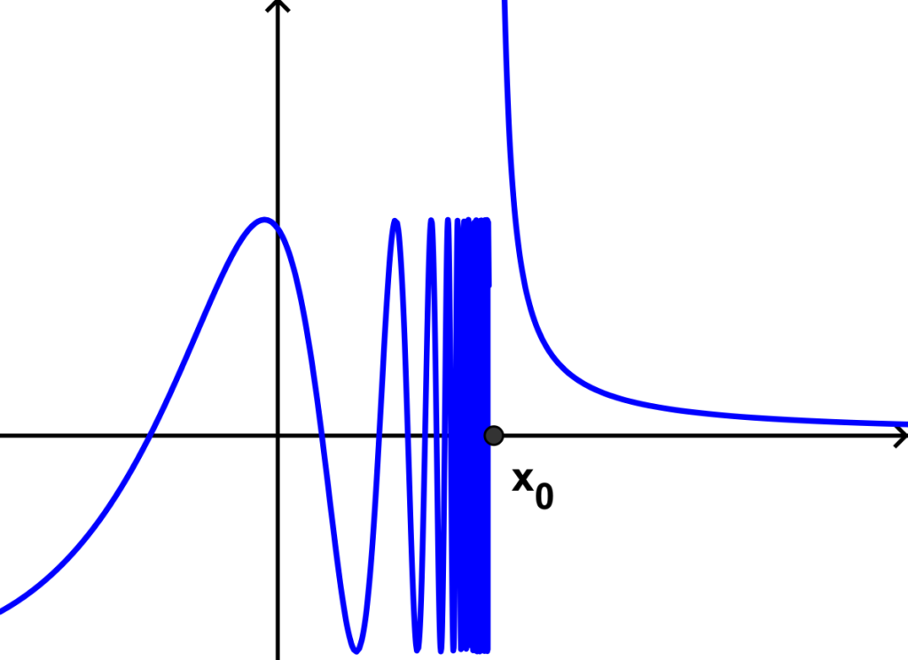
Infinite discontinuity:

We say that a discontinuous graph has an infinite discontinuity at a point $c$ if one or both limits from the left or the right at the point $c$ doesn’t exist, meaning one or both of these limits equal $\pm\infty$ . This type of discontinuity is also called essential discontinuity or discontinuity of the second kind.

Here are some graphs that have infinite discontinuities:

Important results and theorems about continuity

In this section, we are going to take a look at some of the main theorems and results of continuous functions

Definition: Absolute maximum and absolute minimum.

We say that $x^*$ is an absolute maximum of the function $f$ on its domain $D$ , if and only if

$f(x^*)\geq f(x) \;\;\; \forall x\in D$

Respectively, we say that $x^*$ is an absolute minimum of the function $f$ on its domain $D$ , if and only if

$f(x^*)\leq f(x) \;\;\; \forall x\in D$

Now that we defined what is the maximum and the minimum absolute, we can introduce the following theorem:

The theorem of extreme values:

If the function $f: D\to \mathbb{R}$ is continuous and if the domain $D$ is compact, then the function $f$ has an absolute maximum and a minimum absolute on the interval $D$ .

The theorem of indeterminate value

Theorem: Intermediate Value Theorem

Suppose that the function $f:[a,b]\to \mathbb{R}$ is continuous and that $f(a)<\alpha <f(b)$ , then there exists a real number $c\in[a;b]$ which verifies that $f(c)=\alpha$ .

Respectively, is we have that $f$ is continuous and if $(a)>\beta >f(b)$ , then there exists a real number $d\in [a,b]$ which verifies that $f(d)=\beta$ .

This theorem has a very important corollaries, here is one for example:

Corollary:

Suppose that $f:[a,b]\to \mathbb{R}$ is a continuous function; Let:

$m=\min \lbrace f(x) : x \in [a,b]\rbrace$ and $M=Max \lbrace f(x) : x \in [a,b]\rbrace$

Thus for every $\omega\in [m;M]$ there exists $c\in [a,b]$ which verifies that $f(c)=\omega$ .

Also, we can deduce from the theorem of intermediate value that if a function $f$ is continuous on the interval $[a,b]$ , and if $f(a)$ and $f(b)$ have different signs (one is positive and the other is negative) then we know for sure that the function $f$ has at least one root $r$ which is contained in the interval $[a;b]$ this result is also known as the “Bolzano’s theorem”.

Theorem: Bolzano’s Theorem (1817)

If a continuous function defined on an interval is sometimes positive and sometimes negative, it must be 0 at some point.

Theorem:

Suppose that $f : [a,b] \to \mathbb{R}$ is a strictly increasing and a continuous function on the interval $[a,b]$ , and let $c=f(a)$ and $d=f(b)$ , then $f$ is, one to one, $f([a,b])=[c,d]$ ; and the inverse function $f^{-1}$ defined on $[c,d]$ by

$f^{-1}(f(x))=x \;\text{ Where }\; x \in [a,b]$

Is also a continuous function with the domain $[c,d]$ and to its image $[a,b]$ .

Conclusion

Well, here we finish our journey for this time in the world of calculus; we learned in this article about the concept of continuity of a function both at a point or on an interval, we saw the definition of continuity and the condition for with which we can determine if a function is continuous at a given point, not just that we also presented the main properties of continuity since they are essential and important to quickly and easily tell if a function is continuous or not; after that, we presented the meaning of discontinuity and the different types of discontinuity and how to detect them visually just by looking at the graph of the function in question, all of this alongside some examples and illustrations for a better understanding. We also learned some important theorems and results like the theorem of indeterminate value and some important results that we can extract from it. Well, it’s true that we have come to the end of this fun blog post but don’t worry at all, we still are just scratching the surface of Calculus and there is an infinity of things to learn, and we will continuously keep doing that!!!!!

In the meantime, you can take a look at some articles about limits and infinity like Limit of a function: Introduction, Limits of a function: Operations and Properties, Limits of a function: Indeterminate Forms, or the ones about Infinity: Facts, mysteries, paradoxes, and beyond or check the ones about Probability: Introduction to Probability Theory, or Probability: Terminology and Evaluating Probabilities or maybe the one about Probability theory – Conditional Probability!!!!! !!!!!

There are also some articles about Set Theory like Set Theory: Introduction, or Set theory: Venn diagrams and Cardinality!!!!!

Also, if you want to learn more fun subjects, check the post about Functions and some of their properties, or the one about How to solve polynomial equations of first, second, and third degrees!!!!!

And don’t forget to join us on our Facebook page for any new articles and a lot more!!!!!

← PREVIOUS NEXT →

Continuity – Calculus

Introduction

Continuity of a function

Continuity of a function at a point

The tree conditions of continuity at a point:

Continuity of a function on an interval:

Some properties of continuity

Continuity of some known continuous functions:

Discontinuity of a function

Examples of discontinuous functions:

Types of discontinuity:

Jump discontinuity:

Removable discontinuity:

Infinite discontinuity:

Important results and theorems about continuity

The theorem of indeterminate value

Conclusion

Blog Main

Categories

Recent Posts

Archives

Archives

Categories

Meta